Smart charging

The smart charging concept is widely used in different fields and applications. In flextools package, we define smart charging as a tool to coordinate individual EV charging sessions in order to obtain the optimal aggregated demand profile according to a certain objective. There are different scheduling methods to coordinate each session, such as:

• Postpone: shifting charging start time over time
• Interrupt: stop charging during certain time
• Curtail: limiting charging power during certain time

At the same time, the charging sessions can be coordinated with different objectives or goals, such as minimizing the interaction with the power grid, minimizing the energy cost, participating in flexibility or imbalance markets, not surpassing grid constraints or capacity limits, accomplishing with demand-response programs, etc.

The function smart_charging() aims to provide a framework to simulate any of these situations to analyze the impact and benefits of electric vehicle flexibility.

Smart charging algorithm

We have divided the smart charging algorithm contained inside smart_charging() function in two different stages:

1. Setpoint calculation for the aggregated EV demand curve
2. Scheduling of the individual sessions to match the setpoint of the aggregated demand

Below, we will briefly explain the process performed in each one of theses steps.

Setpoint calculation

The setpoint for the aggregated EV demand is understood as the desired, optimal or allowed power demand, depending on the objective and characteristics of the control over the charging points.

Currently, flextools allows the following methods to define the setpoint of the aggregated EV demand:

• Setpoint as maxium EV demand: a maximum EV demand capacity profile can be configured as a constrain to coordinate charging sessions below the limits. This must be set for every EV user profile in the charging sessions data set.

• Setpoint as optimal EV demand: the optinal EV demand is calculated based on a Quadratic programming optimization to minimize the interaction with the power grid (see Net power optimization), the energy cost (see Energy cost optimization) or both (see Combined optimization), setting the parameter opt_objective accordingly. Internally, the smart_charging() function is making use of the optimize_demand() function internally, using parameters direction="forward" to postpone EV sessions and time_horizon=NULL to exploit their flexibility until the end of the optimization window.

Scheduling algorithm

The scheduling method is defined by the parameter method in the smart_charging() function, which can be "postpone", "curtail", "interrupt" or "none". If method = "none", the sessions schedule is not modified and the calculated setpoints are returned as a optimal results. If method is different than "none", after obtaining the setpoint $O_t$ (i.e. optimal load), the scheduling algorithm follows the sequence below for every time slot $t$:

1. Calculate $LF_t$, the EV demand (i.e. flexible load)

2. Get the time slots where $LF_t > O_t$

3. Stop if no more flexibility is required

4. For every time slot where $LF_t > O_t$

   4.1. Get the power difference between load and setpoint in the time slots where $LF_t > O_t$

   4.2. Select flexible sessions (see definition below) and set a priority order

   4.3. Go to next time slot if no more flexibility is available

   4.4. Coordinate flexible sessions to match the setpoint

5. Stop if no more flexibility is available

6. Return the new schedule of EV sessions

To classify a connected EV as a flexible session or not, the flextools package defines the following conditions according to smart charging method used:

• Postpone: the EV has not started charging yet, and the energy required can be charged during the rest of the connection time at the nominal charging power. From all flexible sessions in a time slot, the ones connecting earlier will have priority over the later sessions.
• Interrupt: the charge is not completed yet, and the energy required can be charged during the rest of the connection time at the nominal charging power. From all flexible sessions in a time slot, the ones that have been charging during less time will have priority over the sessions that have been already charging (rotation system).
• Curtail: the charge is not completed yet or will not be completed in the current time slot, and the energy required can be charged during the rest of the connection time at a lower power than the nominal charging power.

The energy and power constraints of these conditions can also be defined in function smart_charging() with the parameters energy_min and charging_power_min, representing the minimum allowed ratios of the nominal values. More information about using these parameters can be found in article Advanced smart charging.

Smart charging examples

Below, some examples of smart_charging() are illustrated for both the grid congestion simulation, where we set a maximum EV capacity to not surpass, and the optimization simulation, where the net power usage or/and the energy cost are optimized thanks to smart charging.

For the smart charging examples that require optimizing the EV demand, a building demand, a solar PV production and energy prices are obtained from the example energy_profiles object provided by flextools:

energy_data <- flextools::energy_profiles %>% 
  filter(isoweek(datetime) == 18, wday(datetime, week_start = 1) <= 5) %>% 
  mutate(
    solar = solar*4,
    building = building*2
  )
head(energy_data)

## # A tibble: 6 × 7
##   datetime            solar building price_imported price_exported price_turn_up
##   <dttm>              <dbl>    <dbl>          <dbl>          <dbl>         <dbl>
## 1 2023-05-01 00:00:00     0     3.06         0.0999          0.025        0.104 
## 2 2023-05-01 00:15:00     0     2.98         0.0999          0.025        0.0993
## 3 2023-05-01 00:30:00     0     2.90         0.0999          0.025        0     
## 4 2023-05-01 00:45:00     0     2.82         0.0999          0.025        0     
## 5 2023-05-01 01:00:00     0     2.74         0.0955          0.025        0     
## 6 2023-05-01 01:15:00     0     2.64         0.0955          0.025        0     
## # ℹ 1 more variable: price_turn_down <dbl>

On top of these energy variables, we can simulate some charging sessions using the evsim package, which provides the function evsim::get_custom_ev_model to create a custom EV model to later simulate EV sessions with evsim::simulate_sessions() function.

We can create an EV model with custom time-cycles and user profiles. In this case, we will consider just one EV user profile (see the EV user profile concept from package evprof), “HomeEV”, which will represent a “charge-at-home” pattern starting in average at 18:00 until next morning.

# For workdays time cycle
workdays_parameters <- dplyr::tibble(
  profile =  "HomeEV",
  ratio = 100,
  start_mean = 18,
  start_sd = 3,
  duration_mean = 13,
  duration_sd = 1,
  energy_mean = 15,
  energy_sd = 2
)

# For weekends time cycle
weekends_parameters <- dplyr::tibble(
  profile = "HomeEV",
  ratio = 100,
  start_mean = 12,
  start_sd = 2,
  duration_mean = 3,
  duration_sd = 2,
  energy_mean = 4,
  energy_sd = 1
)

parameters_lst <- list(workdays_parameters, weekends_parameters)

# Get the whole model
ev_model <- get_custom_ev_model(
  names = c("Workdays", "Weekends"),
  months_lst = list(1:12, 1:12),
  wdays_lst = list(1:5, 6:7),
  parameters_lst = parameters_lst,
  connection_log = FALSE,
  energy_log = FALSE,
  data_tz = "Europe/Amsterdam"
)

Once we have our own model, we simulate 5 sessions per day of our user profile called “HomeEV”, charging at 3.7 kW, during the first 3 days of the energy_data and with a resolution of 15 minutes:

set.seed(123)
ev_sessions <- simulate_sessions(
  evmodel = ev_model, 
  sessions_day = tibble(time_cycle = c("Workdays", "Weekends"), n_sessions = c(5, 5)),
  user_profiles = NULL,
  charging_powers = tibble(power = 3.7, ratio = 1), 
  dates = unique(date(energy_data$datetime))[1:3], 
  resolution = 15
) %>% 
  filter(Profile == "HomeEV")

Session	Timecycle	Profile	ConnectionStartDateTime	ConnectionEndDateTime	ChargingStartDateTime	ChargingEndDateTime	Power	Energy	ConnectionHours	ChargingHours
S1	Workdays	HomeEV	2023-05-01 13:45:00	2023-05-02 03:46:00	2023-05-01 13:45:00	2023-05-01 18:20:00	3.7	17.02	14.02	4.60
S2	Workdays	HomeEV	2023-05-01 14:00:00	2023-05-02 04:33:00	2023-05-01 14:00:00	2023-05-01 17:06:00	3.7	11.47	14.55	3.10
S3	Workdays	HomeEV	2023-05-01 14:15:00	2023-05-02 03:01:00	2023-05-01 14:15:00	2023-05-01 17:42:00	3.7	12.80	12.77	3.46
S4	Workdays	HomeEV	2023-05-01 17:30:00	2023-05-02 07:09:00	2023-05-01 17:30:00	2023-05-01 21:45:00	3.7	15.76	13.65	4.26
S5	Workdays	HomeEV	2023-05-01 21:45:00	2023-05-02 11:47:00	2023-05-01 21:45:00	2023-05-02 01:40:00	3.7	14.54	14.03	3.93
S6	Workdays	HomeEV	2023-05-02 10:15:00	2023-05-02 23:13:00	2023-05-02 10:15:00	2023-05-02 15:01:00	3.7	17.65	12.97	4.77
S7	Workdays	HomeEV	2023-05-02 17:45:00	2023-05-03 05:54:00	2023-05-02 17:45:00	2023-05-02 21:36:00	3.7	14.28	12.15	3.86
S8	Workdays	HomeEV	2023-05-02 19:30:00	2023-05-03 09:18:00	2023-05-02 19:30:00	2023-05-02 23:16:00	3.7	13.99	13.80	3.78
S9	Workdays	HomeEV	2023-05-02 22:45:00	2023-05-03 10:30:00	2023-05-02 22:45:00	2023-05-03 03:28:00	3.7	17.50	11.75	4.73
S10	Workdays	HomeEV	2023-05-02 23:45:00	2023-05-03 13:37:00	2023-05-02 23:45:00	2023-05-03 04:11:00	3.7	16.43	13.87	4.44
S11	Workdays	HomeEV	2023-05-03 11:45:00	2023-05-04 02:00:00	2023-05-03 11:45:00	2023-05-03 14:40:00	3.7	10.80	14.25	2.92
S12	Workdays	HomeEV	2023-05-03 18:00:00	2023-05-04 10:15:00	2023-05-03 18:00:00	2023-05-03 21:47:00	3.7	14.02	16.25	3.79
S13	Workdays	HomeEV	2023-05-03 18:30:00	2023-05-04 07:48:00	2023-05-03 18:30:00	2023-05-03 22:49:00	3.7	15.98	13.30	4.32
S14	Workdays	HomeEV	2023-05-03 20:45:00	2023-05-04 10:00:00	2023-05-03 20:45:00	2023-05-04 01:08:00	3.7	16.24	13.25	4.39
S15	Workdays	HomeEV	2023-05-03 23:00:00	2023-05-04 13:15:00	2023-05-03 23:00:00	2023-05-04 02:51:00	3.7	14.25	14.25	3.85

Finally we can calculate the time-series power demand from each EV with function evsim::get_demand(), using parameter by="Sessions":

ev_demand <- ev_sessions %>% 
  get_demand(by = "Session") 

ev_demand %>% 
  plot_ts(ylab = "Power demand (kW)", stackedGraph = T, fillGraph = T)

It is visible that these EV users tend to coincide during the evening peak hours while, if they were coordinated, they could make a more efficient usage of the power grid. Following, you will find some examples about how to coordinate these EV sessions using smart_charging() but first of all let’s start with a minimal example.

Let’s simulate smart charging with:

• Optimization objective “grid” (minimizing interaction with the grid)
• Scheduling method “curtail” (reducing charging power when required)
• no contextual data for optimization (opt_data will be just a date time sequence)
• optimization window: starting at 6:00AM and with a length of 1 day (24h)

sc_results <- smart_charging(
  ev_sessions, 
  opt_data = tibble(datetime = ev_demand$datetime, production = 0),
  opt_objective = "grid",
  method = "curtail",
  window_days = 1,
  window_start_hour = 6
)

The object returned by function smart_charging() is always list with 3 more objects:

names(sc_results)

## [1] "sessions"  "setpoints" "demand"    "log"

• setpoints: time-series data frame with the optimal setpoints of the EV demand
• sessions: coordinated EV sessions’ data frame according to the setpoint
• log: list with messages about the smart charging algorithm (flexibility needs and availability, sessions modified, etc.). This is empty by default and filled with messages when include_log = TRUE.

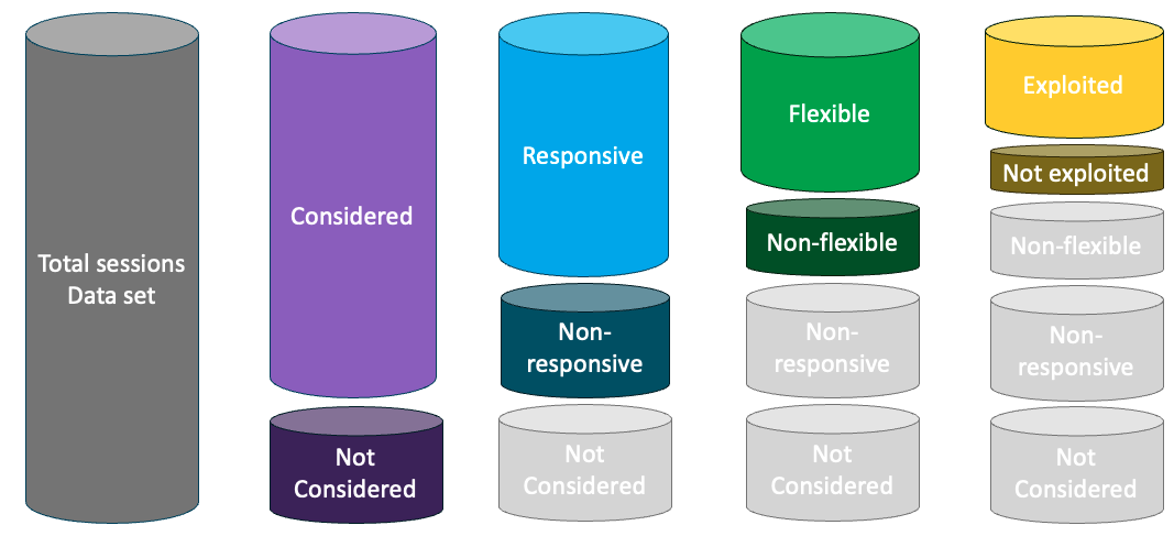
Moreover, if we print the results we see a summary of the charging sessions that have been participating in the smart charging program, differentiating them between Considered, Responsive, Flexible and Exploited:

print(sc_results)

## Smart charging results as a list of 3 objects: charging sessions, user profiles setpoints and log messages.
## Simulation from 2023-05-01 to 2023-05-05 with a time resolution of 15 minutes.
## For this time period, there were 3 smart charging windows, where:
##   - 15 sessions were considered ( 100 % of total data set).
##   - 15 sessions were Responsive ( 100 % of considered sessions).
##   - 15 sessions were Flexible ( 100 % of responsive sessions).
##   - 15 sessions were Exploited ( 100 % of flexible sessions).

This classification is done by the smart charging algorithm according to the optimization window hours, the method and the sessions’ features:

• Considered: charging sessions that charge within the optimization windows and are not considered outliers (their connection times fit the 95% percentile).
• Responsive: charging sessions that accept to participate in the smart charging program. The ratio of responsive sessions from every EV user profile is configured with the responsive parameter.
• Flexible: charging sessions that are flexible in a specific time slot. This depends on the session’s features and the scheduling method (as described in the Scheduling algorithm section).
• Exploited: charging sessions that have been modified in a a specific time slot.

The following figure illustrates the classification of sessions according to smart charging program participation:

Also note that after applying the smart charging, the sessions object from the results has more rows than the original sessions object. It is not the number of total charging sessions that has increased, but all flexible sessions have been divided in multiple time slots. This allows to modify the charging power of every time slot to 0 (postpone or interrupt methods) or between 0 and the nominal power (curtail method).

In the following example you can see how Session “S1” has a different Power value in different time slots:

head(sc_results$sessions) %>% 
  knitr::kable(caption = "Coordinated charging sessions")

Coordinated charging sessions

Session	Timecycle	Profile	ConnectionStartDateTime	ConnectionEndDateTime	ChargingStartDateTime	ChargingEndDateTime	Power	Energy	ConnectionHours	ChargingHours	Responsive	Flexible	Exploited	EnergyLeft	ConnectionHoursLeft
S1	Workdays	HomeEV	2023-05-01 13:45:00	2023-05-01 14:00:00	2023-05-01 13:45:00	2023-05-01 14:00:00	3.70	0.92	0.25	0.25	TRUE	TRUE	FALSE	17.02	14.02
S1	Workdays	HomeEV	2023-05-01 14:00:00	2023-05-01 14:15:00	2023-05-01 14:00:00	2023-05-01 14:15:00	2.21	0.55	0.25	0.25	TRUE	TRUE	TRUE	16.09	13.77
S1	Workdays	HomeEV	2023-05-01 14:15:00	2023-05-01 17:30:00	2023-05-01 14:15:00	2023-05-01 17:30:00	1.47	4.79	3.25	3.25	TRUE	TRUE	TRUE	15.54	13.52
S1	Workdays	HomeEV	2023-05-01 17:30:00	2023-05-01 19:15:00	2023-05-01 17:30:00	2023-05-01 19:15:00	1.10	1.93	1.75	1.75	TRUE	TRUE	TRUE	10.75	10.27
S1	Workdays	HomeEV	2023-05-01 19:15:00	2023-05-01 21:45:00	2023-05-01 19:15:00	2023-05-01 21:45:00	1.10	2.76	2.50	2.50	TRUE	TRUE	TRUE	8.82	8.52
S1	Workdays	HomeEV	2023-05-01 21:45:00	2023-05-01 22:30:00	2023-05-01 21:45:00	2023-05-01 22:30:00	0.88	0.66	0.75	0.75	TRUE	TRUE	TRUE	6.06	6.02

Then, the setpoints object from the result is a tibble that represents the objective EV demand and the power profile that the algorithm tried to match while scheduling the EV sessions:

head(sc_results$setpoints)

## # A tibble: 6 × 2
##   datetime            HomeEV
##   <dttm>               <dbl>
## 1 2023-05-01 00:00:00      0
## 2 2023-05-01 00:15:00      0
## 3 2023-05-01 00:30:00      0
## 4 2023-05-01 00:45:00      0
## 5 2023-05-01 01:00:00      0
## 6 2023-05-01 01:15:00      0

We can visualise the setpoint on top to the EV demand to see how the optimal EV demand is different to the original demand:

ev_demand %>% 
  left_join(
    rename(sc_results$setpoints, Setpoint = HomeEV),
    by = "datetime"
  ) %>% 
  plot_ts(ylab = "Power (kW)", legend_show = "onmouseover") %>% 
  dyStackedRibbonGroup(unique(ev_sessions$Session)) %>% 
  dySeries("Setpoint", color = "red", strokePattern = "dashed", strokeWidth = 2)

We can visualize the difference between the defined setpoint and the final EV user profile by applying the native plot() function to the smart_charging() results, which is equivalent to use the function plot_smart_charging(). Moreover, to see the difference between the flexible and the original EV demand, we can pass the sessions parameter to the plot() function.

plot(sc_results, sessions = ev_sessions)

In this case, we see that at the end of the optimization window we have some peaks because the EVs have to charge their energy requirements before the end of the window. For methods to solve this issue see the section “The EV demand is pushed to the end of the optimization window” in the Advanced smart charging article.

Finally, the log object from the results is a list of strings containing all log messages from scheduling charging sessions for every timestamp and EV user profile. To enable the log messages it is required to configure the parameter log = TRUE in smart_charging() function.

Grid capacity limit

Imagine that we have to charge the example EV charging sessions in an installation that has a maximum grid connection of 8 kW:

grid_capacity <- 8

ev_demand %>% 
  plot_ts(ylab = "Power demand (kW)", stackedGraph = T, fillGraph = T, legend_show = "onmouseover") %>% 
  dyLimit(grid_capacity, "Grid capacity", color = "red")

Since our peak goes above 18kW, we need to use smart charging to allow the EV users to charge under the grid capacity. In order to define a grid capacity in the smart_charing() function, a column with "grid_capacity" name must be found in the opt_data parameter:

opt_data <- tibble(
  datetime = ev_demand$datetime, # Same date-time sequence than the demand
  grid_capacity
)
head(opt_data)

## # A tibble: 6 × 2
##   datetime            grid_capacity
##   <dttm>                      <dbl>
## 1 2023-05-01 00:00:00             8
## 2 2023-05-01 00:15:00             8
## 3 2023-05-01 00:30:00             8
## 4 2023-05-01 00:45:00             8
## 5 2023-05-01 01:00:00             8
## 6 2023-05-01 01:15:00             8

Also, the parameter opt_objective must be set to "none" in order to skip optimization, since the setpoint for the smart charging algorithm will be given by the opt_data column named “HomeEV”.

Then, which smart charging method should we use? Let’s compare them, considering optimization windows of 24 hours from 6:00AM to 6:00AM.

First we can try with the postpone strategy setting method="postpone":

sc_results <- ev_sessions %>% 
  smart_charging(
    opt_data = opt_data, 
    opt_objective = "none",
    method = "postpone",
    window_days = 1, 
    window_start_hour = 6
  )

## Warning: `production` variable not found in `opt_data`. No local energy production will be considered.

ev_demand_opt <- sc_results$sessions %>% 
  get_demand(by = "Session") 

ev_demand_opt %>% 
  plot_ts(ylab = "Power demand (kW)", stackedGraph = T, fillGraph = T, legend_width = 150) %>% 
  dyLimit(grid_capacity, "Grid capacity", color = "red") %>% 
  dyAxis("y", valueRange = c(0, 10))

We see that the later EV sessions have been shifted during the night instead of start charging right at the connection time during peak hours. This is not a problem if all EVs are completely charged during their connection times, but it may suppose a risk for the late EV connections that have to wait until all previous sessions have been charged. This issue is solved with the interrupt strategy, where a rotation system is designed to charge a similar amount of energy to all connected EVs.

Let’s see the difference with method="interrupt":

sc_results <- ev_sessions %>% 
  smart_charging(
    opt_data = opt_data, 
    opt_objective = "none",
    method = "interrupt",
    window_days = 1, 
    window_start_hour = 6
  )

## Warning: `production` variable not found in `opt_data`. No local energy production will be considered.

ev_demand_opt <- sc_results$sessions %>% 
  get_demand(by = "Session") 

ev_demand_opt %>% 
  plot_ts(ylab = "Power demand (kW)", stackedGraph = T, fillGraph = T, legend_width = 150) %>% 
  dyLimit(grid_capacity, "Grid capacity", color = "red") %>% 
  dyAxis("y", valueRange = c(0, 10))

Now we see the same aggregated result but we also see that the individual sessions are interrupted to enable new sessions to charge, for a better equality among EV users. However, both postpone and interrupt methods do not provide high flexibility in terms of power since the individual charging power can’t be reduced. In that sense, the curtail method provides a higher flexibility potential to adapt the EV demand to more variable or fluctuating signals such as flexibility markets or energy prices.

Let’s see the difference with method="curtail":

sc_results <- ev_sessions %>% 
  smart_charging(
    opt_data = opt_data, 
    opt_objective = "none",
    method = "curtail",
    window_days = 1, 
    window_start_hour = 6
  )

## Warning: `production` variable not found in `opt_data`. No local energy production will be considered.

ev_demand_opt <- sc_results$sessions %>% 
  get_demand(by = "Session") 

ev_demand_opt %>% 
  plot_ts(ylab = "Power demand (kW)", stackedGraph = T, fillGraph = T, legend_width = 150) %>% 
  dyLimit(grid_capacity, "Grid capacity", color = "red") %>% 
  dyAxis("y", valueRange = c(0, 10))

Now we see that the EV demand is completely adapted to the grid capacity, sharing the full capacity among all different charging EVs in equal parts.

Net power optimization

Imagine the EV charging sessions from our examples in a building that has it own demand profile and PV production. We can use the example data set from energy_data to visualize it:

ev_demand <- get_demand(ev_sessions)

energy_data %>% 
  left_join(ev_demand, by = "datetime") %>% 
  select(-starts_with("price")) %>% 
  plot_ts(ylab = "Power (kW)", strokeWidth = 2) %>% 
  dySeries("solar", "PV production", "orange") %>% 
  dyStackedRibbonGroup(c("HomeEV","building"), color = c("purple", "navy"))

We see that the EV demand cause an even higher demand peak during the evening peak hours. To solve this issue, the EV sessions can be coordinated with the building demand profile to obtain a lower aggregated peak. This can be done with function smart_charging(), using a net power optimization (i.e. opt_objective = "grid", see more information in Net power optimization article. We will simulate it using a "curtail" method, considering optimization windows of 24 hours from 6:00AM to 6:00AM, and renaming the variable "solar" to "production" and "building" to "static" in the opt_data object:

opt_data <- energy_data %>% 
  rename(production = solar, static = building)

sc_results <- ev_sessions %>% 
  smart_charging(
    opt_data = opt_data, 
    opt_objective = "grid",
    method = "curtail",
    window_days = 1, 
    window_start_hour = 6
  )

## Warning: Unknown or uninitialised column: `sessions`.

## Warning: Unknown or uninitialised column: `demand`.

## Warning: Unknown or uninitialised column: `log`.

plot(sc_results, sessions = ev_sessions)

We see that the EVs in this case could match the setpoint during most of the time. The optimal setpoint is a specific power curve calculated to obtain the flattest possible net power curve. We can check that by adding the flexible EV profiles to the building (consumption = building + HomeEV) and visualizing the net power profile with function plot_net_power(), which calculates the net power from columns consumption and production.

ev_demand_flex <- sc_results$sessions %>% 
  get_demand() 

df_flex <- energy_data %>% 
  select(datetime, building, solar) %>% 
  left_join(
    ev_demand_flex, by = "datetime"
  ) %>% 
  mutate(
    consumption = building + HomeEV,
    production = solar
  )

plot_net_power(df_flex)

From this graph we see that during the evening peak, the demand can be completely flat, shaving the peak, if the EVs can be coordinated to match the setpoint. We can also compare the net power profile from the static and flexible case with the parameter original_df. In this plot we clearly see the added value of EV flexibility to reduce the impact to the grid during the evening peak.

df_static <- energy_data %>% 
  select(datetime, building, solar) %>% 
  left_join(
    ev_demand, by = "datetime"
  ) %>% 
  mutate(
    consumption = building + HomeEV,
    production = solar
  )

plot_net_power(df_flex, original_df = df_static)

However, we see that during some timeslots the EV demand surpasses the setpoint. This happens in order to charge all energy requirements for all EVs, since by default energy_min = 1. If we set energy_min = 0.5, we see that we can meet the setpoint to all time slots but not all energy required is charged to the vehicles.

sc_results <- ev_sessions %>% 
  smart_charging(
    opt_data = opt_data, 
    opt_objective = "grid",
    method = "curtail",
    window_days = 1, 
    window_start_hour = 6,
    energy_min = 0.5
  )

## Warning: Unknown or uninitialised column: `sessions`.

## Warning: Unknown or uninitialised column: `demand`.

## Warning: Unknown or uninitialised column: `log`.

plot(sc_results, sessions = ev_sessions)

Energy cost optimization

As we have seen, the EV demand from our “HomeEV” user profile occur mainly during evening peak hours, which is a problem for grid congestion but also for the EV user since they are also the most expensive hours (with dynamic tariffs):

energy_data %>% 
  select(
    datetime, solar, building, price_imported, price_exported
  ) %>% 
  left_join(ev_demand, by = "datetime") %>% 
  plot_ts(strokeWidth = 2) %>% 
  dyAxis("y", "Power (kW)") %>% 
  dyAxis("y2", "Price (€/kWh)") %>% 
  dyStackedRibbonGroup(c("HomeEV","building"), color = c("purple", "navy")) %>% 
  dySeries("solar", "PV production", "orange") %>% 
  dySeries("price_imported", "Imported energy price", axis = "y2", color = "red", strokePattern = "dashed") %>% 
  dySeries("price_exported","Exported energy price",  axis = "y2", color = "green", strokePattern = "dashed")

The energy cost can be optimized with function smart_charging(), using energy cost optimization (i.e. opt_objective = "cost", see more information in Energy cost optimization article. We will simulate it using a "curtail" method, considering optimization windows of 24 hours from 6:00AM to 6:00AM, and renaming the variable "solar" to "production" and "building" to "static" in the opt_data object, and keeping the price_imported and price_exported variables:

opt_data <- energy_data %>% 
  select(
    datetime, production = solar, static = building, 
    price_imported, price_exported
  )
head(opt_data)

## # A tibble: 6 × 5
##   datetime            production static price_imported price_exported
##   <dttm>                   <dbl>  <dbl>          <dbl>          <dbl>
## 1 2023-05-01 00:00:00          0   3.06         0.0999          0.025
## 2 2023-05-01 00:15:00          0   2.98         0.0999          0.025
## 3 2023-05-01 00:30:00          0   2.90         0.0999          0.025
## 4 2023-05-01 00:45:00          0   2.82         0.0999          0.025
## 5 2023-05-01 01:00:00          0   2.74         0.0955          0.025
## 6 2023-05-01 01:15:00          0   2.64         0.0955          0.025

sc_results <- ev_sessions %>% 
  smart_charging(
    opt_data = opt_data, 
    opt_objective = "cost",
    method = "curtail",
    window_days = 1, 
    window_start_hour = 6
  )

## Warning: Unknown or uninitialised column: `sessions`.

## Warning: Unknown or uninitialised column: `demand`.

## Warning: Unknown or uninitialised column: `log`.

plot(sc_results)

In this case the setpoint gets very high values when the price_imported variable has low values. We have 2 options to solve that:

1. Use a lambda value
2. Use a combined optimization

In this case we will use a combined optimization, setting the parameter opt_objective = 0.1 meaning 90% cost minimization and 10% net power minimization:

sc_results <- ev_sessions %>% 
  smart_charging(
    opt_data = opt_data, 
    opt_objective = 0.1,
    method = "curtail",
    window_days = 1, 
    window_start_hour = 6
  )

## Warning: Unknown or uninitialised column: `sessions`.

## Warning: Unknown or uninitialised column: `demand`.

## Warning: Unknown or uninitialised column: `log`.

plot(sc_results, sessions = ev_sessions)

We can visualize the difference on the energy cost thanks to the optimization using function plot_energy_cost(). This function requires a data frame with the total consumption and production, as well as the price_imported and price_exported variables. Moreover, we can compare the static and flexible cases by using the original_df parameter.

ev_demand_flex <- sc_results$sessions %>% 
  get_demand() 

df_flex <- energy_data %>% 
  select(datetime, building, solar, price_imported, price_exported) %>% 
  left_join(
    ev_demand_flex, by = "datetime"
  ) %>% 
  mutate(
    consumption = building + HomeEV,
    production = solar
  )

df_static <- energy_data %>% 
  select(datetime, building, solar, price_imported, price_exported) %>% 
  left_join(
    ev_demand, by = "datetime"
  ) %>% 
  mutate(
    consumption = building + HomeEV,
    production = solar
  )

plot_net_power(df_flex, original_df = df_static)

From this graph we see that the demand has been shifted from the evening peak to the night valley, looking for cheaper hours. We can check the difference in the total energy cost by using get_energy_total_cost() function:

• Total energy cost of static scenario:

get_energy_total_cost(df = df_static)

## [1] 168.7046

• Total energy cost of flexible scenario:

get_energy_total_cost(df = df_flex)

## [1] 155.8546

Energy cost with grid constraints

Even though we can talk about two different objectives, there could be a situation where we want to minimize the energy cost under certain grid constraints. In these cases, the optimization objective should be “cost” as well, but we can make use of the grid_capacity variable configurable in the opt_data parameter from smart_charging() function.

The grid_capacity variable in the opt_data tibble represents the maximum consumption, not only for the EV demand but also the rest of static demand (consumption = building + EV):

df_static <- energy_data %>% 
  left_join(ev_demand, by = "datetime") %>% 
  mutate(
    consumption = building + HomeEV,
    production = solar
  )

plot_net_power(df_static)

So let’s assume that for the current demand we have a grid capacity of 10 kW. We can visualize with the import_capacity parameter in the plot_net_power() function to see if the net power surpasses the grid capacity:

plot_net_power(df_static, import_capacity = 10)

Then we can perform a cost optimization with the parameter opt_objective = 0.1 meaning 90% cost minimization and 10% net power minimization. For that, we will also include the grid_capacity variable in the opt_data object:

opt_data <- energy_data %>% 
  select(
    datetime, production = solar, static = building, 
    price_imported, price_exported
  ) %>% 
  mutate(
    grid_capacity = 10
  )
head(opt_data)

## # A tibble: 6 × 6
##   datetime            production static price_imported price_exported
##   <dttm>                   <dbl>  <dbl>          <dbl>          <dbl>
## 1 2023-05-01 00:00:00          0   3.06         0.0999          0.025
## 2 2023-05-01 00:15:00          0   2.98         0.0999          0.025
## 3 2023-05-01 00:30:00          0   2.90         0.0999          0.025
## 4 2023-05-01 00:45:00          0   2.82         0.0999          0.025
## 5 2023-05-01 01:00:00          0   2.74         0.0955          0.025
## 6 2023-05-01 01:15:00          0   2.64         0.0955          0.025
## # ℹ 1 more variable: grid_capacity <dbl>

sc_results <- ev_sessions %>% 
  smart_charging(
    opt_data = opt_data, 
    opt_objective = 0.1,
    method = "curtail",
    window_days = 1, 
    window_start_hour = 6
  )

## Warning: Unknown or uninitialised column: `sessions`.

## Warning: Unknown or uninitialised column: `demand`.

## Warning: Unknown or uninitialised column: `log`.

df_flex <- energy_data %>% 
  left_join(sc_results$setpoints, by = "datetime") %>% 
  mutate(
    consumption = building + HomeEV,
    production = solar
  )

plot_net_power(df_flex, original_df = df_static)

Now we see that our total consumption remains below the limits of our grid capacity. But is the cost being optimized?

plot_energy_cost(df_flex, original_df = df_static)

It seems that we consume more during valley hours (night) than during peak hours (evening), so the cost could be still decreased. We can check the difference in the total energy cost by using get_energy_total_cost() function:

• Total energy cost of static scenario:

get_energy_total_cost(df = df_static)

## [1] 168.7046

• Total energy cost of flexible scenario:

get_energy_total_cost(df = df_flex)

## [1] 14747588325

In this case, the cost optimization is not possible if the grid is constrained.