Advanced smart charging • flextools

The smart_charging() function provides some parameters that may not be required in most of simulations but configuring them in specific cases can make a huge difference. This article raises some cases where a more advanced knowledge and configuration of these parameters may be required to obtain the desired results.

For the smart charging examples in this article, the same example data sets energy_data and ev_sessions from the article Smart charging will be used:

head(energy_data)

## # A tibble: 6 × 7
##   datetime            solar building price_imported price_exported price_turn_up
##   <dttm>              <dbl>    <dbl>          <dbl>          <dbl>         <dbl>
## 1 2023-05-01 00:00:00     0     3.06         0.0999          0.025        0.104 
## 2 2023-05-01 00:15:00     0     2.98         0.0999          0.025        0.0993
## 3 2023-05-01 00:30:00     0     2.90         0.0999          0.025        0     
## 4 2023-05-01 00:45:00     0     2.82         0.0999          0.025        0     
## 5 2023-05-01 01:00:00     0     2.74         0.0955          0.025        0     
## 6 2023-05-01 01:15:00     0     2.64         0.0955          0.025        0     
## # ℹ 1 more variable: price_turn_down <dbl>

head(ev_sessions)

## # A tibble: 6 × 11
##   Session Timecycle Profile ConnectionStartDateTime ConnectionEndDateTime
##   <chr>   <chr>     <chr>   <dttm>                  <dttm>               
## 1 S1      Workdays  HomeEV  2023-05-01 13:45:00     2023-05-02 03:46:00  
## 2 S2      Workdays  HomeEV  2023-05-01 14:00:00     2023-05-02 04:33:00  
## 3 S3      Workdays  HomeEV  2023-05-01 14:15:00     2023-05-02 03:01:00  
## 4 S4      Workdays  HomeEV  2023-05-01 17:30:00     2023-05-02 07:09:00  
## 5 S5      Workdays  HomeEV  2023-05-01 21:45:00     2023-05-02 11:47:00  
## 6 S6      Workdays  HomeEV  2023-05-02 10:15:00     2023-05-02 23:13:00  
## # ℹ 6 more variables: ChargingStartDateTime <dttm>, ChargingEndDateTime <dttm>,
## #   Power <dbl>, Energy <dbl>, ConnectionHours <dbl>, ChargingHours <dbl>

For all smart charging simulations the following parameters will be considered:

scheduling method: curtail
optimization window days: 1
optimization window start hour: 6:00 AM

The EV demand is pushed to the end of the optimization window

Usually applying the smart_charging() function with default configuration will not prevent that some EV users surpass their setpoints, due to a lack of flexibility from the EV sessions. When this happens, normally it results in a higher demand at the end of the optimization window because the smart charging algorithm tries to match the setpoint until there’s no more flexibility from the EV users and the EV must be charged.

Below, we will see examples of these situations for the 2 types of setpoints that smart_charging() function can consider (grid capacity setpoint and optimization setpoint), and how to deal with that.

Setpoint as grid capacity

Imagine that there’s a maximum grid connection has to be reduced to 4 kW, so that we can charge only one EV at a time:

grid_capacity <- 4

We configure this grid capacity as a setpoint for the EV user profile:

opt_data <- tibble(
  datetime = ev_demand$datetime, # Same date-time sequence than the demand
  HomeEV = grid_capacity
)
head(opt_data)

## # A tibble: 6 × 2
##   datetime            HomeEV
##   <dttm>               <dbl>
## 1 2023-05-01 00:00:00      4
## 2 2023-05-01 00:15:00      4
## 3 2023-05-01 00:30:00      4
## 4 2023-05-01 00:45:00      4
## 5 2023-05-01 01:00:00      4
## 6 2023-05-01 01:15:00      4

sc_results <- smart_charging(
  sessions = ev_sessions,
  opt_data = opt_data, 
  opt_objective = "none",
  method = "curtail",
  window_days = 1, 
  window_start_hour = 6
)

## Warning: `production` variable not found in `opt_data`. No local energy production will be considered.

plot(sc_results, sessions = ev_sessions)

The demand is being postponed by the smart charging algorithm to match the setpoint during all possible hours, but when the end of the optimization window is reaching, the vehicle must charge to accomplish with the energy requirements by the EV user. This means that all EV users are not able to charge all their requirements under these grid conditions.

Therefore, in these scenarios where the grid stability is the priority we have to assume that not all EV can be completely charged, and we should be able to simulate this impact to the EV user. This scenario can be configured with the parameter energy_min, as the required minimum ratio of the energy required by the EV user. With energy_min = 0 the algorithm considers that EVs may disconnect without charging all their energy requirements, while with energy_min = 1 the algorithm will make sure that all EV users charge their energy requirements, even though the setpoint is not achieved.

Let’s try a value of energy_min = 0 to see how the algorithm works and the corresponding impact to the vehicles:

sc_results <- smart_charging(
  sessions = ev_sessions,
  opt_data = opt_data, 
  opt_objective = "none",
  method = "curtail",
  window_days = 1, 
  window_start_hour = 6,
  energy_min = 0
)

## Warning: `production` variable not found in `opt_data`. No local energy production will be considered.

plot(sc_results, sessions = ev_sessions)

Now we see that the grid capacity constraint is completely respected. But at which price?

We can calculate the impact on the EV user in terms of percentage of energy charged with the function summarise_energy_charged():

summarise_energy_charged(sc_results, sessions = ev_sessions) %>% 
  knitr::kable(caption = "Percentage of energy charged (%)")

Percentage of energy charged (%)
Session	EnergyRequired	EnergyCharged	PctEnergyCharged
S1	17.02	16.16	95
S2	11.47	11.47	100
S3	12.80	12.71	99
S4	15.76	NA	NA
S5	14.54	NA	NA
S6	17.65	17.65	100
S7	14.28	14.28	100
S8	13.99	NA	NA
S9	17.50	NA	NA
S10	16.43	NA	NA
S11	10.80	10.80	100
S12	14.02	NA	NA
S13	15.98	NA	NA
S14	16.24	NA	NA
S15	14.25	NA	NA

We see that, to achieve our setpoint, some EV users can only charge a bit more than the 50% of their energy requirements.

We can also check that setting energy_min = 0.7, for example, results in surpassing the setpoint again, but all EV users charge at least a 70% of their energy requirements:

sc_results <- smart_charging(
  sessions = ev_sessions,
  opt_data = opt_data, 
  opt_objective = "none",
  method = "curtail",
  window_days = 1, 
  window_start_hour = 6,
  energy_min = 0.7
)

## Warning: `production` variable not found in `opt_data`. No local energy production will be considered.

plot(sc_results, sessions = ev_sessions)

summarise_energy_charged(sc_results, sessions = ev_sessions) %>% 
  knitr::kable(caption = "Percentage of energy charged (%) - `energy_min = 0.7`")

Percentage of energy charged (%) - `energy_min = 0.7`
Session	EnergyRequired	EnergyCharged	PctEnergyCharged
S1	17.02	16.16	95
S2	11.47	11.47	100
S3	12.80	12.71	99
S4	15.76	NA	NA
S5	14.54	NA	NA
S6	17.65	17.65	100
S7	14.28	14.28	100
S8	13.99	NA	NA
S9	17.50	NA	NA
S10	16.43	NA	NA
S11	10.80	10.80	100
S12	14.02	NA	NA
S13	15.98	NA	NA
S14	16.24	NA	NA
S15	14.25	NA	NA

Setpoint as optimal demand

Let’s consider a grid optimization for our EV demand in the context of the following energy flows:

energy_data %>% 
  left_join(ev_demand, by = "datetime") %>% 
  select(-starts_with("price")) %>% 
  plot_ts(ylab = "Power (kW)", strokeWidth = 2) %>% 
  dySeries("solar", color = "orange") %>% 
  dyStackedRibbonGroup(c("HomeEV","building"), color = c("purple", "navy"))

ev_sessions %>% 
  smart_charging(
    opt_data = energy_data %>% rename(static = building, production = solar), 
    opt_objective = "grid",
    method = "curtail",
    window_days = 1, 
    window_start_hour = 6
  ) %>% 
  plot()

## Warning: Unknown or uninitialised column: `sessions`.

## Warning: Unknown or uninitialised column: `demand`.

## Warning: Unknown or uninitialised column: `log`.

From the plot above we see that during most of the time the EV demand can be adapted to the setpoint but in the second optimization window, the EV demand that is not charged during the morning has to be charged during the night surpassing the setpoint.

If the setpoint is calculated for an optimization objective (e.g. "grid" or "cost"), then surpassing the setpoint may not suppose a risk but only a not optimal solution. Even though, situations like the one above should be avoided since we can have a rebound effect at the end of the optimization window. A solution to these situations is the parameter power_th, which allows a certain threshold between the setpoint value and the EV demand in every time slot. See the application of power_th = 0.05 to allow a threshold of 5% of the setpoint:

ev_sessions %>% 
  smart_charging(
    opt_data = energy_data %>% rename(static = building, production = solar), 
    opt_objective = "grid",
    method = "curtail",
    window_days = 1, 
    window_start_hour = 6,
    power_th = 0.05
  ) %>% 
  plot()

## Warning: Unknown or uninitialised column: `sessions`.

## Warning: Unknown or uninitialised column: `demand`.

## Warning: Unknown or uninitialised column: `log`.

The EV model has a minimum charging power

It is known that some EV models have a minimum charging power, so below this power they can’t be charged at all. Therefore, a possible solution is to specify a minimum charging power with the parameter charging_power_min. When charging_power_min = 0 and method = "curtail", the charging power can be reduced until 0 kW (interrupted), while a value of charging_power_min = 0.5 would only allow curtailing the EV charging power until the 50% of its nominal charging power.

Let’s simulate that all EVs must charge at least at a 30% of their power requirements:

sc_results <- ev_sessions %>% 
  smart_charging(
    opt_data = energy_data %>% rename(static = building, production = solar), 
    opt_objective = "grid",
    method = "curtail",
    window_days = 1, 
    window_start_hour = 6,
    charging_power_min = 0.3
  )

## Warning: Unknown or uninitialised column: `sessions`.

## Warning: Unknown or uninitialised column: `demand`.

## Warning: Unknown or uninitialised column: `log`.

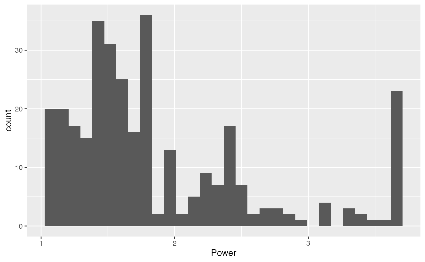
Check that the minimum power of the Exploited sessions (i.e. the ones that provided flexibility) corresponds to the 30% of 3.7 (1.11kW):

sc_results$sessions %>% 
  filter(Exploited) %>% 
  pull(Power) %>% 
  min()

## [1] 1.11

We can also make a histogram to show the distribution of charging power values. It is visible that the limit of 30% of the nominal power (1.11 kW) is actually limiting the flexibility, since a lot of sessions have been charged at this minimum charging rate:

sc_results$sessions %>% 
  filter(Exploited) %>% 
  ggplot(aes(Power)) + 
  geom_histogram()

## `stat_bin()` using `bins = 30`. Pick better value with `binwidth`.

Histogram of charging power values And if we compare the final EV demand with the setpoint, in general we see a good result even though the setpoint is not achieved during the most restrictive periods:

plot(sc_results)