Parallel processing

The function smart_charging() has complex calculations (described in the Smart charging article) that are repeated on a daily basis. A 24 hours period is considered an independent optimization window, thus the corresponding calculations can be done in parallel.

In computer science, a common practice to reduce computation times is parallel processing when the CPU of the computer has multiple cores that can work independently. We can discover the number of cores in our computer CPU using function parallel::detectCores():

n_cores <- parallel::detectCores()
print(n_cores)

## [1] 14

In this case, the CPU used is the Apple M4 Pro, which features 10 performance CPU cores (P-core) running at up to 4.5 GHz along with 4 efficient cores (E-core) running at up to 2.6 GHz. So, when parallel::detectCores() returns 14, macOS is exposing 14 logical cores — but not all of them are equal in speed.

In flextools, parallel processing is used inside the smart_charging() function, using the mirai package and its mirai::daemons() function to set the number of cores that we want to work in parallel. Below you will find an example about how to use this functionality.

Smart charging

Package evsim provides a sample data set of California EV sessions from October 2018 to September 2021. If we filter sessions corresponding to 2019, we have >15.000 sessions, with an average of 70 charging sessions during working days.

sessions_2019 <- evsim::california_ev_sessions_profiles %>% 
  filter(year(ConnectionStartDateTime) == 2019)

Let’s use these real charging sessions to simulate smart_charging() using multiple cores (with mirai::daemons()) but also different values of number of days (optimization windows):

n_days_seq <- c(3, 7, 15, 30, 180, 365) # Days in a year
n_cores_seq <- c(1, seq(2, 10, 2)) # 10 performance cores (P-core)
cores_time <- tibble(
  days = rep(n_days_seq, each = length(n_cores_seq)),
  cores = rep(n_cores_seq, length(n_days_seq)), 
  time = 0
)

for (nd in n_days_seq) {
  message(nd, " days ---------------- ")
  sessions <- sessions_2019 %>%
    filter(date(ConnectionStartDateTime) <= dmy(01012019)+days(nd)) %>% 
    evsim::adapt_charging_features(time_resolution = 15)

  sessions_demand <- evsim::get_demand(sessions, resolution = 15)
  
  opt_data <- tibble(
    datetime = sessions_demand$datetime,
    production = 0
  )
  
  for (mcc in cores_time$cores[cores_time$days == nd]) {
    message(mcc, " cores")
    if (mcc > 1) {
      mirai::daemons(mcc)
    }
    
    results <- system.time(
      smart_charging(
        sessions, opt_data, opt_objective = "grid", method = "curtail",
        window_days = 1, window_start_hour = 5
      )
    )
    mirai::daemons(0)
    
    cores_time$time[
      cores_time$cores == mcc & cores_time$days == nd
    ] <- as.numeric(results[3])
  }
}

# Adapt variables for a better plot
cores_time <- cores_time %>% 
    mutate(
      days = factor(
        paste(days, "days"), 
        levels = factor(paste(n_days_seq, "days"))
      ), 
      cores = factor(cores)
    )

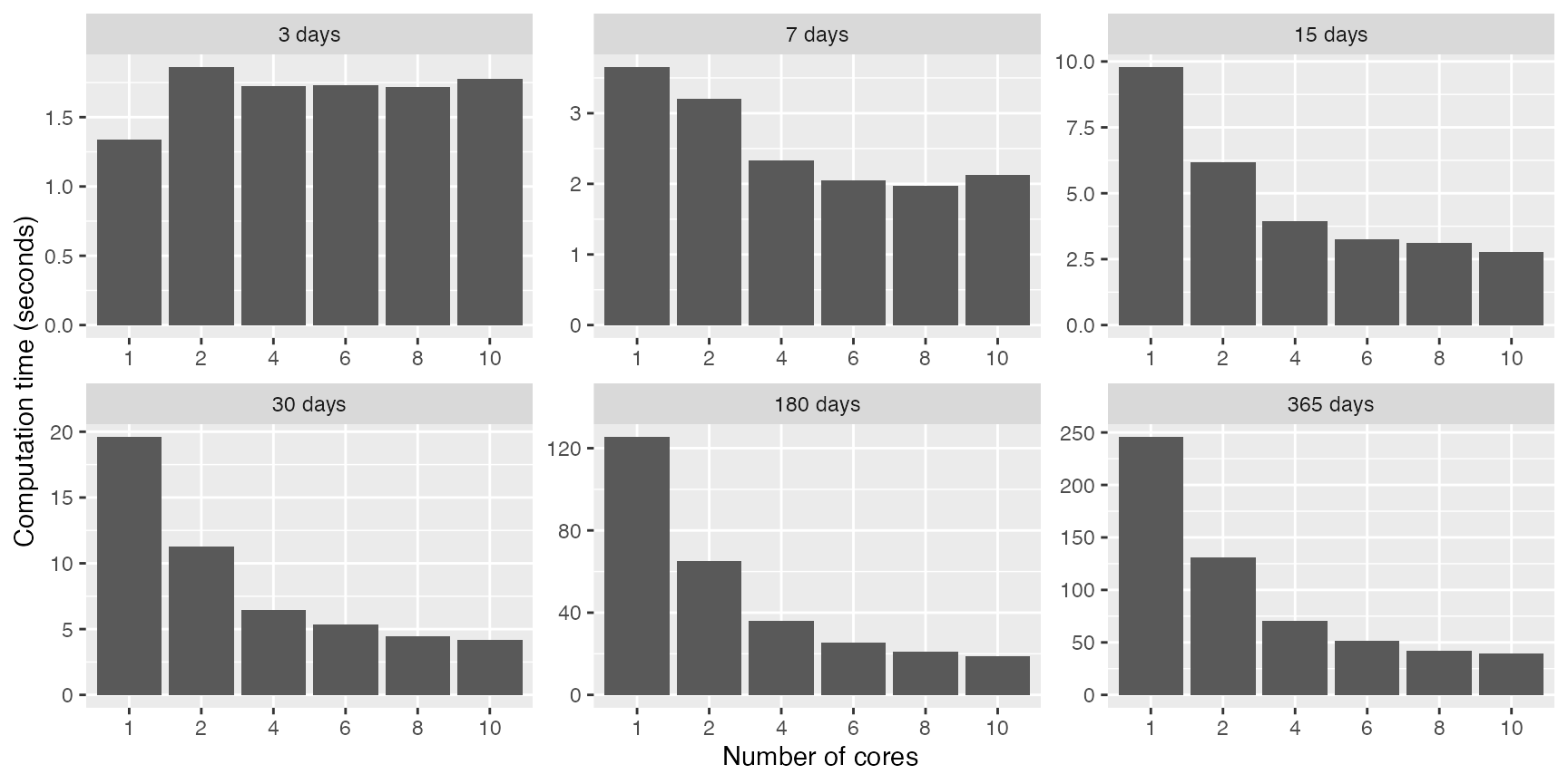
And below there’s the plot of the results, were we can see:

1. Parallel processing is only useful from 1 week of data
2. From more than 1 month of data the computation time is reduced at a half with just 2 cores, and then the decrease of computation time is less relevant.

cores_time %>%
  ggplot(aes(x = cores, y = time)) +
  geom_col() + 
  labs(x = "Number of cores", y = "Computation time (seconds)") + 
  facet_wrap(vars(days), scales = "free", nrow = 2)