Outliers detection

As explained, the clustering method used in package evprof is Gaussian Mixture Models clustering. This method is sensible to outliers since it tries to explain as most as possible all the variance of the data, which results to wide and non-specific Gaussian distributions (clusters). Therefore evprof package provides different functions to detect and filter outliers. At the same time, it is also recommended to perform the clustering process in a logarithmic scale, to include negative values to originally positive variables. The logarithmic transformation can be done in most of functions, setting the log argument to TRUE.

Here we have a set of sessions of example, noisy_set:

noisy_set <- sessions_divided %>% # Obtained from the "Get started" article
  filter(Disconnection == "Home", Timecycle == "Friday") # Friday Home

plot_points(noisy_set, size = 0.2)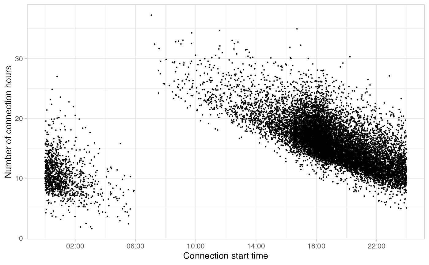

We set the start parameter at 06:00:

options(
  evprof.start.hour = 6
)

And we can plot it in logarithmic scale to visualize the areas of the plot where outliers are:

plot_points(noisy_set, size = 0.2, log = T)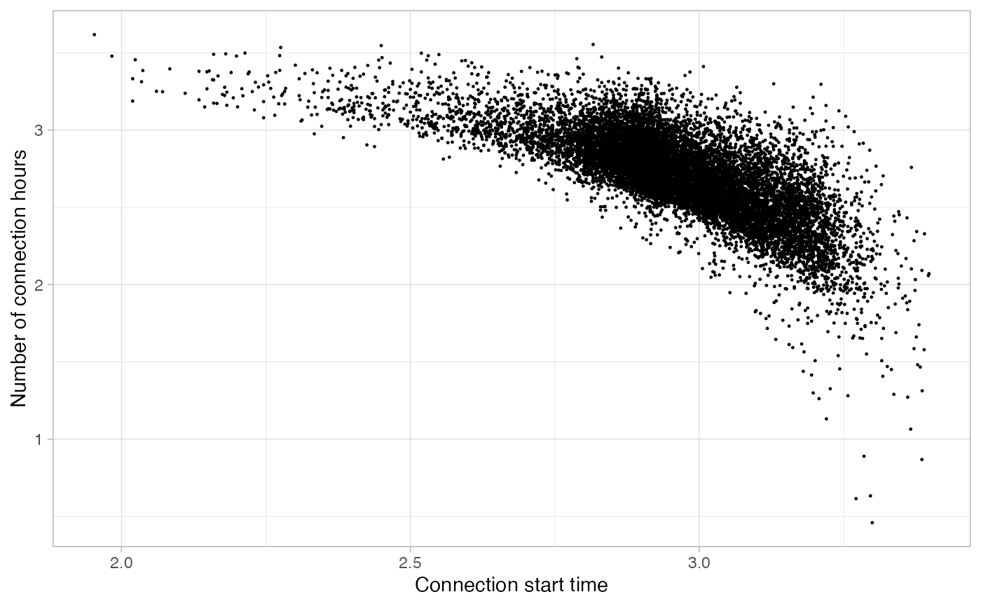

Cutting sessions

If we see a part of the graph that consists clearly of outlying points, then we can cut directly the sessions below or above this specific limit using the function cut_sessions(). This function lets to configure the Connection Duration limits (connection_hours_min and connection_hours_max) and the Connection Start limits (connection_start_min and connection_start_max). If we want to make the division in logarithmic scale it is important to set the argument log = TRUE.

noisy_set <- noisy_set %>% 
  cut_sessions(connection_hours_min = 1.5, connection_start_min = 2.5, log = T)

plot_points(noisy_set, size = 0.2, log = T)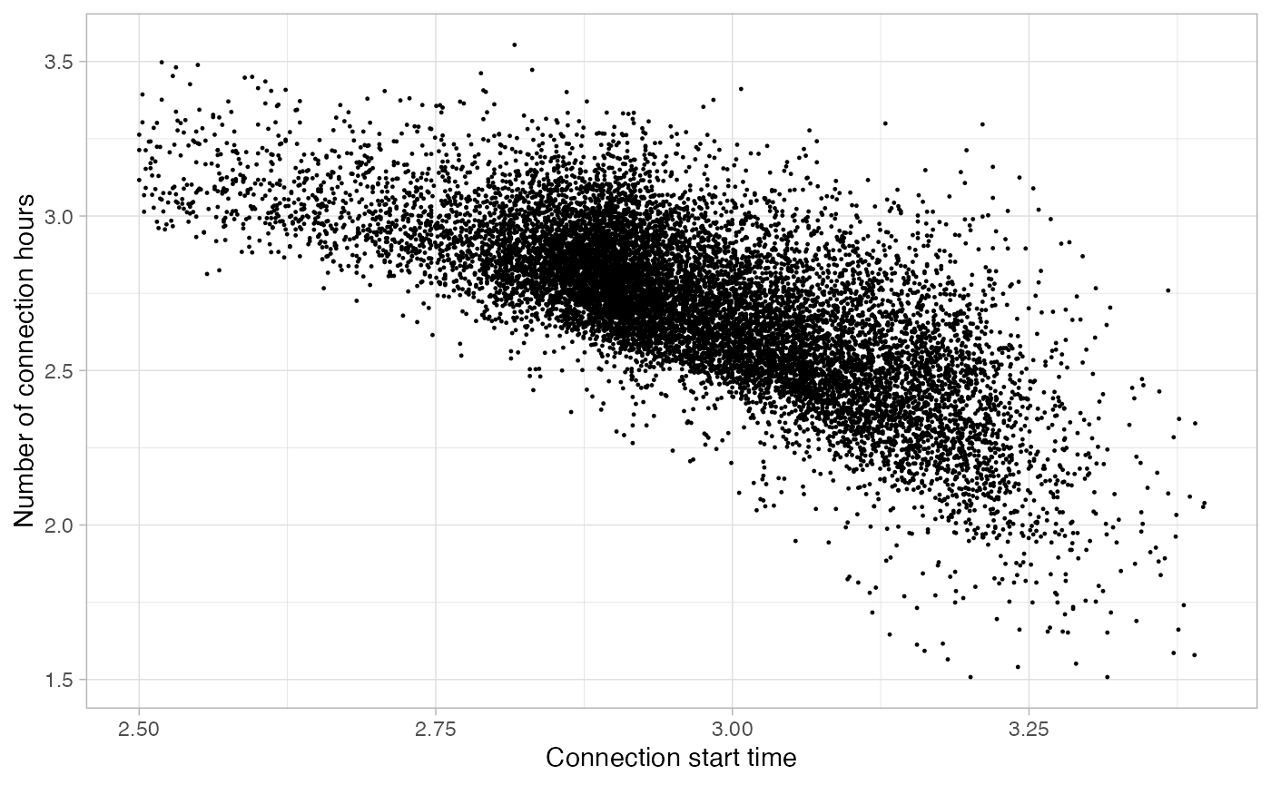

Noise cleaning with DBSCAN clustering

The DBSCAN (Density-based spatial clustering of applications with noise) clustering method is widely used for dividing data sets according to density zones. In this case, this method has been used to detect the outliers, i.e the data points outside of the main density zones. Package evprof proposes the function detect_outliers with the purpose of classify a certain noise threshold of noise. The main arguments of this function are MinPts, eps (DBSCAN parameters) and noise_th (noise threshold, in %). The function detect_outliers allows you to configure just the MinPts and noise_th to automatically find the eps value.

Usually values around of MinPts = 200 and noise_th = 2 are recommended, but you could configure an iteration to find the best combination according to the plot obtained with function plot_outliers. First, let’s create a table with all combinations of MinPts and noise_th values you want:

.MinPts <- c(10, 50, 100, 200)
.noise_th <- c(1, 3, 5, 7)
dbscan_params <- tibble(
  MinPts = rep(.MinPts, each = length(.noise_th)),
  noise_th = rep(.noise_th, times = length(.MinPts))
)

print(dbscan_params)

Now let’s run the iteration to create a plot for every combination (using purrr::pmap function):

plots_list <- pmap(
  dbscan_params,
  ~ noisy_set %>% 
  detect_outliers(MinPts = ..1, noise_th = ..2, log = T) %>% 
  plot_outliers(log = T, size = 0.2) + 
    theme(legend.position = "none")
)

You can save the plots in a pdf for a proper visualization, using cowplot::plot_grid function.

ggsave(
  filename = 'my_noise_detection.pdf', 
  plot = cowplot::plot_grid(
    plotlist = plots_list, nrow = 4, ncol = 4, labels = as.list(rep(.MinPts, each = length(.noise_th)))
  ),
  width = 500, height = 250, units = "mm"
)

From all these plots, we see that the the higher the MinPts is, the more center-focused is the final clean cluster. This is not a valid approach for all data sets, so the value of MinPts must be defined properly in every case. In this case, we decide that a good compromise solution is a value of MinPts of 200 and a noise threshold of 5%:

plots_list[[15]]